

Predict Expected Loss Costs
Overview
Business Problem
The insurance industry is highly regulated in the US, especially for lines of businesses that are mandatory; this means individuals and businesses are legally required to purchase insurance. Personal auto is one such example, where insurance carriers strive to refine their pricing plan to increase pricing accuracy, improve profitability, and minimize the potential of adverse selection. The personal auto insurance market is also highly competitive, with insurers looking to gain an edge on every business aspect, from marketing, risk selection, and pricing, to efficient claim handling. Among these many aspects, accurate pricing has paramount importance. Generalized linear models (GLMs) have risen in popularity for personal auto insurance pricing since the 1990s because of its flexible structure and interpretability; however, GLMs have their own limitations for insurance applications such as requiring manual processes for interaction identification and feature selection. Intense competition and the low cost associated with customers switching carriers have pressured insurers to turn to machine learning models to determine a more accurate price commensurate with an individual policyholder’s risk and exposure.
Intelligent Solution
AI and machine learning models present an incredible opportunity for building accurate personal auto insurance pricing models. Models are capable of calculating loss cost estimates based on large amounts of policyholder data. They learn from historical loss cost data and help the insurer analyze the increasingly complex relationship between loss cost and policy/driver/vehicle attributes as well many other features accessible to the insurer. Using and assessing large amounts of features, models can automatically identify/incorporate interactions among the different features. In less regulated markets, loss cost models have already proven to effectively differentiate costs between high and low risk policyholders, leading to more accurate and personalized pricing for personal auto insurance policies.
In highly regulated markets such as the US, insurers have started adopting machine learning models to assist their refined pricing efforts. These models can be fed to a pricing plan via rating tables or be incorporated in the pricing plan via risk tiers. There are many additional applications of loss cost model predictions—such as guiding marketing and underwriting, or identifying high and low profitability segments of an insurer’s book of business. Regulators are gaining comfort with machine learning models for insurance pricing and discussions have been ongoing around regulating machine learning pricing models (1).
Value Estimation
What has ROI looked like for this use case?
Depending on the complexity of existing pricing models and current marketing and underwriting processes, insurers relying on machine learning models have reportedly achieved an improvement of combined loss ratio of 1% to 2%. For a personal auto book of business of $1 billion annual written premium, this amounts to an improvement in profit of $100–200 million. Besides the measurable benefit, these models also enhance an insurer’s understanding of the underlying businesses to promote a much healthier book of business, which potentially helps sustainable growth and profitability in the long run.
Technical Implementation
About the Data
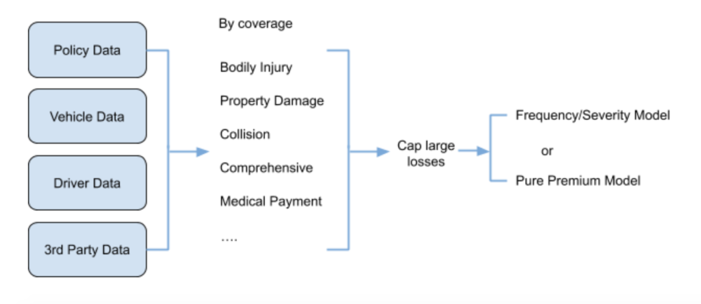
For this tutorial, we are relying on a synthetic dataset that resembles personal auto insurance pricing for collision coverage. As a common practice, personal auto insurance pricing is conducted by coverage, e.g., Bodily Injury, Property Damage, Collision and Comprehensive. Therefore, historical data should be split by coverage before model training.
Insurance losses often exhibit heavily skewed distributions, with fat right tails. To prevent those rare but extremely large losses from biasing the model, it is common practice to cap losses by coverage at a specified threshold (e.g., 99th percentile). Details on constructing the dataset are provided in the next section. The focus of this use case will be collision coverage, where losses are already capped.
Problem Framing
The target variable to build a loss cost model is IncurredClaims; and because this is a numeric target this is a regression problem.
The features below represent some of the predictor variables an insurer would likely use to develop loss cost models. The data spans across claims, policy, vehicle, and 3rd party information. Exposure represents the earned exposure amount for each policy record in the dataset.
Since the data for this use case has been simplified for demonstration purposes, an insurance company’s actual pricing dataset will often include many additional data elements. Beyond the features listed below, we suggest incorporating any additional data your organization may collect that could be relevant to the use case. As you will see later, DataRobot is able to help you quickly differentiate important vs unimportant features.
Sample Feature List
| Feature | Type | Description | Source |
|---|---|---|---|
| IncurredClaims | Numeric, Target | Total claim paid out during the policy period. | Claims |
| Exposure | Numeric | The period of time that this contract was active. 1 for a full year. < 1 if the contract was cancelled part-way through. | Policy |
| SumInsured | Numeric | The value of the vehicle. | Vehicle |
| NoClaimBonus | Numeric | The premium discount percentage, earned by number of years without reporting a claim. | Policy |
| VehicleMake | Categorical | Name of the vehicle manufacturer. | Vehicle |
| VehicleModel | Categorical | Name of the vehicle model. | Vehicle |
| EngineCapacity | Numeric | Size of the engine in cubic centimetres. | Vehicle |
| VehicleAge | Numeric | Age of the vehicle in years at the time that the contract started. | Vehicle |
| ClientType | Categorical | Whether the customer is a business (“Commercial”) or a human (“Retail”). | Policy |
| DriverAge | Numeric | Age of the youngest driver of the vehicle. No ages are collected for vehicles owned by businesses. | Driver |
| NumberOfDrivers | Numeric | # drivers insured by the policy. | Policy |
| CustomerTenure | Numeric | # years the policy has been with the insurer | Policy |
| Gender | Categorical | Gender of the main driver. C = business. M = male. F = female. | Driver |
| MaritalStatus | Categorical | Marital status of the main driver. | Driver |
| Longitude | Numeric | Longitude of the garaging address | Policy |
| Latitude | Numeric | Latitude of the garaging address | Policy |
| PostCode_Aged_18_24 | Numeric | Proportion of adult population age 18-24 in the garaging zip. | 3rd Party |
| PostCode_Aged_25_29 | Numeric | Proportion of adult population age 25-29 in the garaging zip. | 3rd Party |
| PostCode_Aged_30_39 | Numeric | Proportion of adult population age 30-39 in the garaging zip. | 3rd Party |
| PostCode_Aged_40_44 | Numeric | Proportion of adult population age 40-44 in the garaging zip. | 3rd Party |
| PostCode_Aged_45_49 | Numeric | Proportion of adult population age 45-49 in the garaging zip. | 3rd Party |
| PostCode_Aged_50_59 | Numeric | Proportion of adult population age 50-59 in the garaging zip. | 3rd Party |
| PostCode_Aged_60 | Numeric | Proportion of adult population age 60 or greater in the garaging zip. | 3rd Party |
| PostCode_PersonsPerDwelling | Numeric | Average number of people per dwelling in the garaging zip. | 3rd Party |
| PostCode_annualKm | Numeric | Average number of kilometres driven per annum for vehicles in the garaging zip. | 3rd Party |
| PostCode_VehiclesPerDwelling | Numeric | Average number of vehicles per dwelling in the garaging zip. | 3rd Party |
| PostCode_CommuteViaCar | Numeric | Proportion of the adult population who commute to work via vehicle in the garaging zip. | 3rd Party |
| DistributionChannel | Numeric | The distribution channel via which the insurance policy was sold. | 3rd Party |
| SydneyRegion | Numeric | Whether the address is in the Sydney region. | Policy |
Data Preparation
Here are some considerations that may be helpful in trying to develop a dataset for this use case.
In practice, a typical personal auto insurance carrier stores data at various granularities: policy, driver, vehicle, and claim levels. This data often resides in separate databases, such as a policy admin system, claim admin system, application system, and 3rd party databases. Many of these databases, especially policy and claim systems, are transaction-based.
Within the policy admin system, data is often stored as a single row for each policy period and endorsement. If a policy experiences changes during the policy term, an additional record will be added to the database reflecting the change. Some reasons a policy might experience a change include endorsements or cancellations. The policy database records the policy start date (aka policy effective date), endorsement date, and policy end date (aka policy expiration date). These dates indicate the start and end points for each policy record. The length of time for each policy record is called the exposure amount. Exposure is an important concept for insurance policies as it represents the unit of risk that an insurance policy is covering.
Within the claim admin system, claim payments and reserve change for a specified claim often appear as single records in each database. A claim which closes quickly might only have one record representing a single payment in the database. Other more complex claims may require multiple claim payments over the course of numerous months. Within the database, these claims would be represented by multiple records for each subsequent payment or reserve change. The claim admin system uses the evaluation date to discern these snapshots for every claim.
For loss cost models, it’s very important to use the most recent available evaluation date so that the target will reflect the most up-to-date claim cost. Depending on coverage, claims from most recent policy years may be removed from the modeling dataset due to either the incomplete policy year or immature claims. In addition, models should only include information which was known as-of the point in time at which the model will be creating predictions.
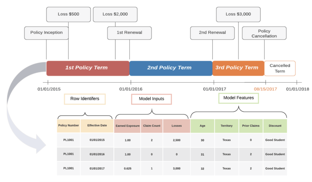
Data from each source needs to be joined into a singular table in order to be ingested by DataRobot for modeling. The visualization illustrates how to convert a policy with three policy terms and multiple losses into a single table.
Model Training
Upload data to DataRobot
DataRobot Automated Machine Learning automates many parts of the modeling pipeline. Instead of hand-coding and manually testing dozens of models to find the one that best fits your needs, DataRobot automatically runs dozens of models and finds the most accurate one for you, all in a matter of minutes.
But before we begin modeling, the data can first be uploaded to DataRobot’s platform in multiple ways, including dragging files onto user interface, searching through local file browser, and fetching from a remote server, local JDBC-enabled databases, or local Hadoop file system. (See this community article for more details.)
Once the modeling data is uploaded to DataRobot, EDA (Exploratory Data Analysis) will be run automatically which produces a brief summary of the data, such as feature type, summary statistics for numeric features, and distribution of each feature. Data quality is checked at this step as well. The guardrails that DataRobot has in place ensure only data with good quality goes into the modeling process.
Model setup
First of all, we need to tell DataRobot what we are predicting; in this use case, it is IncurredClaims. Notice that the IncurredClaims has a typical distribution for insurance losses: a spike at 0 and the rest following a Gamma type of distribution, which is usually described as a zero-inflated distribution. For this type of distribution, DataRobot by default will select Tweedie Deviance as the optimization metric.
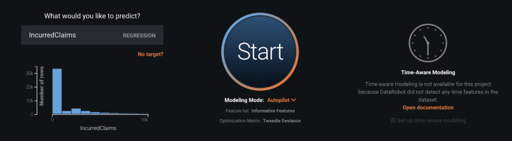
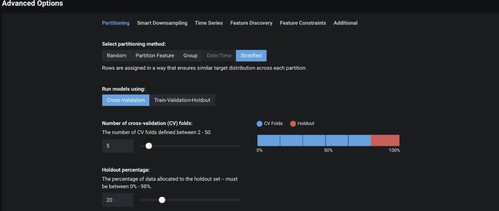
DataRobot’s default model setup applies to many use cases. For example, DataRobot sets aside 20% of the uploaded data as a holdout set and the rest is split into different folds for cross validation or train/validation/test set. This is one of guardrails DataRobot uses to ensure model accuracy while avoiding overfitting.
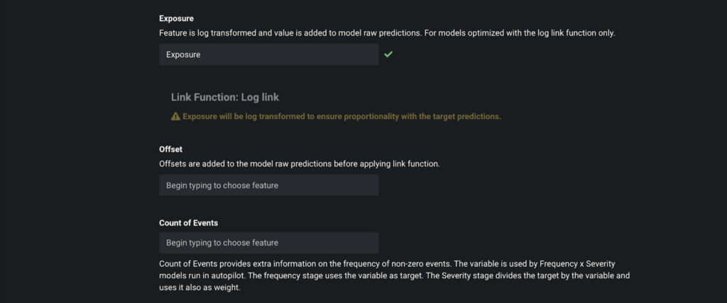
DataRobot also provides advanced settings which are commonly used for insurance loss cost modeling, such as:
- Monotonicity constraints on Feature Constraints tab
- Exposure, Offset, and Count of Events on the Additional tab
For this particular use case, we are going to specify Exposure since each row in our dataset represents different insurance exposures. In this exemplary dataset, Exposure is also the feature name, so we only need to type Exposure in the screen below.
Once all the settings are taken care of, we are ready to click Start to kick-off Autopilot.
Let’s jump to interpreting the model results.
Interpret Results
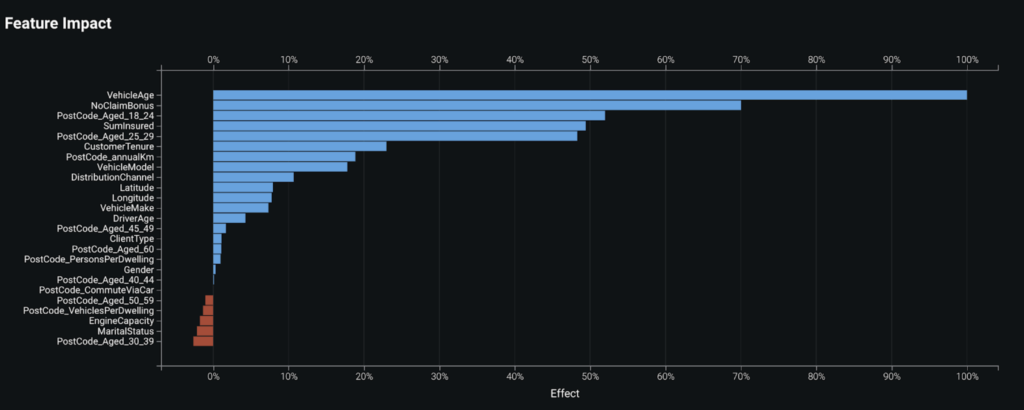
Feature importance
Once a model is built, it is helpful to know which features are the key drivers within our model. The Feature Impact plot ranks features from most important to least important, measuring each feature relative to the top feature. In this example, we can see that VehicleAge is the most important feature for this model, followed by NoClaimBonus, PostCode_Aged_18_24, and SumInsured.
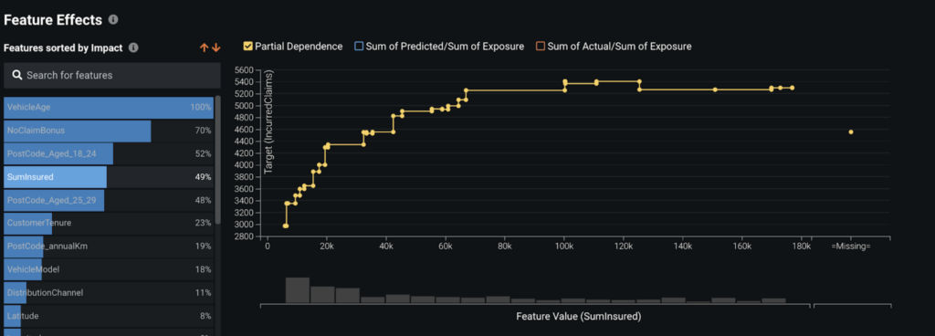
Partial Dependence Plot
Besides understanding which features are important in the model, we’d also like to understand how each feature affects our predictions. This is what the Feature Effects plot is for. In the following screenshot, we can see the partial dependence for the SumInsured variable. We can see that more expensive vehicles tend to be associated with higher loss costs, but the relationship levels off for vehicles worth more than 70K.
Prediction Explanations
Insurance stakeholders need explanations for model predictions. For example, if an underwriter sees a model produce a high-loss cost prediction, their first question will be, “what policy characteristics warrant such a high prediction?”.
Insights at the individual prediction level help an underwriter understand how a prediction is made and enable them to have personalized conversations with customers.
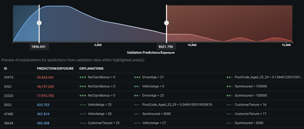
By default, DataRobot provides the top 3 Prediction Explanations for each prediction, but you can request up to 10 explanations. Model predictions and explanations can be downloaded in a CSV file. You also have full control over which predictions will be populated in the downloaded CSV file by specifying the thresholds for high and low predictions.
The graph below shows the top explanations for the 3 highest and 3 lowest predictions. From the graph we can tell that, in general, the high predictions are associated with younger drivers and higher value vehicles; while the low predictions are associated with older and lower value vehicles.
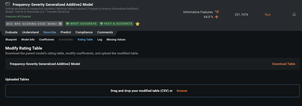
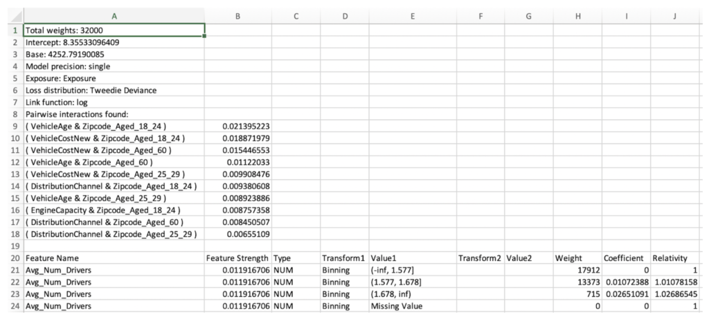
Rating Tables
For certain types of models such as Generalized Additive2 Model (GA2M), DataRobot allows you to download a rating table. GA2M rating tables have a very similar structure to rating tables produced by Generalized Linear Model (GLM)(2).
The advantages of GA2M models:
- Automatically detect pairwise interactions
- Automatically bin numeric variables
- Regularize features to reduce overfitting
In the snippet below, you can find Intercept, Base, Coefficient, and Relativity, where Base and Relativity are simply the exponential of Intercept and Coefficient, respectively, since the link function is log.
One thing that is worth pointing out is that DataRobot does not choose a reference level for Coefficient and Relativity; therefore if a reference level is desired for each feature, your intercept should be adjusted accordingly to reflect the change.
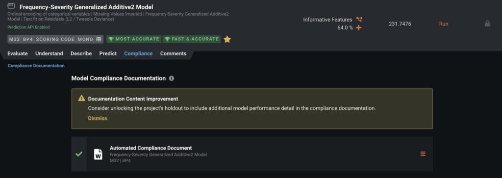
Compliance Documentation
For highly regulated industries like insurance, DataRobot automates many critical compliance tasks associated with developing a model and, by doing so, decreases time-to-deployment. For each model, you can generate individualized documentation to provide comprehensive guidance on what constitutes effective model risk management. Then, you can download the report as an editable Microsoft Word document (DOCX). The generated report includes the appropriate level of information and transparency necessitated to meet regulatory compliance demands.
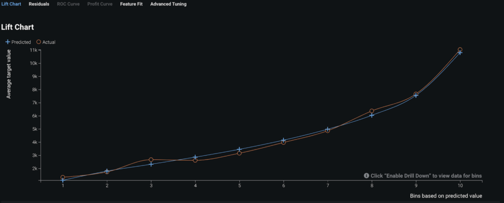
Evaluate Accuracy
DataRobot provides multiple ways to evaluate a model’s performance. The Lift Chart below shows how effective the model is in terms of differentiating policies with lowest risk (on the left) from those with highest risk (on the right). Since the actuals (orange curve) closely tracks the predicted values (blue curve), we know our model fits the data well.
Post-Processing
Depending on the intended purpose, model outputs or model predictions can be used in various ways:
- For actuaries focusing on pricing, relativities from the rating table can be used to create rating factors in a pricing plan.
- For underwriters who are interested in risk selection, the model predictions can be converted to risk scores. For example, the 1st percentile is corresponding to the bottom 1% policies with lowest risk while the 100th percentile represents the top 1% policies with highest risk.
Insurers may wish to compare DataRobot model predictions with their existing pricing plans in order to identify mispriced segments. They can use these insights to refine pricing or simply to guide underwriting and marketing efforts.
Business Implementation
Decision Environment
After you finalize a model, DataRobot makes it easy to deploy the model into your desired decision environment. Decision environments are the methods by which predictions will ultimately be used for decision making.
Decision Maturity
Automation | Augmentation | Blend
The manner in which a loss cost model is deployed depends upon its intended application and can vary by company.
Pricing actuaries may take the relativities from the downloaded rating table to create rating factors for the filing to the insurance department; they may also share the rating factors with the IT department which will then incorporate the factors to the rating engine; this approach relies on the available IT resources and so can be a very lengthy process.
Model Deployment
The preferred approach is:
- Download the rating table from the selected model.
- Modify desired coefficients and relativities within the rating table.
- Upload the modified rating table to DataRobot.
- Build a new DataRobot model using the modified rating table.
- Deploy the final model using a dedicated prediction server (API Deployment).
This approach does not completely eliminate IT involvement, but it can save a lot of time spent on manual coding. API-deployed models also allow performance monitoring through service health, data drift, and accuracy. As predictions are made over time, the model monitoring and management (MMM) function will keep track of all these metrics and alert you of any degradation.
If the model predictions are to be used for risk selection by underwriters, the recommended approach of deployment is an API deployment. An API call from an existing process is needed to pass the data to be scored to the server and return predictions back to the production system, such as PolicyCenter. The predictions can also be fed to dashboard tools like Tableau or Power BI so that hot and cold spots can be visualized by various stakeholders.
Decision Stakeholders
- Pricing actuaries
- Underwriters
- Marketing
- Senior Management
Model Monitoring
Pricing models should be monitored constantly. DataRobot enables the monitoring of the model’s performance from different perspectives, especially data drift. Being able to monitor the distribution of the new business submissions and to compare it with the training data has profound impact on the insurer’s understanding of not only the appropriateness of the pricing model for the new businesses but also its competitive position in the market.
Implementation Risks
- It is critical to ensure that scoring data has similar distribution to the training data which was used to build the model. For real-time scoring, insurers may want to monitor the distribution of new business submissions on a regular basis, such as weekly or monthly. Out-of-time validation is recommended during the model building process as an additional form of model checking. If there are strong trends in overall claims costs, a recalibration process or frequent model retraining may be required.
- The modeling dataset comes from multiple sources, including both internal policy/claim databases and external data. Extreme care should be in place to make sure data from different sources is joined appropriately before being fed to the model for scoring.
- Whenever external data sources are relied on, insurers should be aware of the possibility of downtime for third-party data feeds.
- For features which might change or present new levels, such as zip code (although not very frequently), a catch-all factor should be in place to make sure a new policy can be properly priced.
- Credibility of insurance data should always be evaluated. Certain insurance lines of business may not have enough historical data to provide signal that would warrant the use of a predictive model.
- For implementations with extensive IT involvement, proper lead time should be planned so the pricing model can be integrated into the production system in a timely manner.
Trusted AI
In addition to traditional risk analysis, the following elements of AI Trust may require attention in this use case.
Target leakage: Target leakage describes information that should not be available at the time of prediction being used to train the model. That is, particular features leak information about the eventual outcome that will artificially inflate the performance of the model in training. As mentioned in “Implementation Risks,” this loss-cost modeling dataset comes from multiple sources, and the potential for leakage is one of the risks of improper joins. It is critical to identify the point of prediction and ensure no data be included past that time. DataRobot additionally supports robust target leakage detection in the second round of exploratory data analysis and the selection of the Informative Features feature list during autopilot.

Experience the DataRobot AI Platform
Less Friction, More AI. Get Started Today With a Free 30-Day Trial.
Sign Up for Free
Explore More Use Cases
-
InsurancePredict Policy Churn For New Customers
Ensure the long term profitability of incoming members by predicting whether they will churn within the first 12 months of a policy application.
Learn More -
InsurancePredict Which Insurance Products to Offer
Predict which products are best for cross-selling to drive successful next best offer campaigns
Learn More -
InsurancePredict Claims Litigation
Predict from first notice of loss which claims have a high risk of going to litigation.
Learn More -
InsurancePredict Individual Loss Development
Predict loss development on every individual claim based on their unique attributes.
Learn More